With the rapid advancement of AI technologies, an increasing number of fields have begun incorporating AI to achieve more accurate and efficient analytical results. One emerging discipline is computational pathology, which integrates AI algorithms with pathology to analyze medical data at scale.

In pathology, abundant data—such as genomic profiles, clinical reports, and histology images—can be processed using machine learning to extract meaningful patterns relevant for research and clinical practice. When medical experts interpret AI-processed data, they gain clearer and more precise insights. With AI assisting the analysis of large, complex datasets, clinicians are able to uncover subtle patterns that may otherwise be overlooked, ultimately improving diagnostic speed and accuracy.

This article introduces an AI model designed for analyzing pathology images: Clustering-constrained Attention Multiple-Instance Learning (CLAM). CLAM automatically identifies regions with important pathological features within a whole-slide image (WSI) and performs automated classification. In tumor pathology, for example, CLAM can distinguish normal from abnormal tissue and pinpoint the evidence used for its prediction. Beyond obtaining a classification result, users can also evaluate whether the model’s reasoning aligns with known pathology or reveals new underlying patterns.

To use CLAM, pathologists simply provide WSI files (.svs, .ndpi, .tiff, etc.), biopsy images, or microscopic images along with their corresponding labels. CLAM can achieve high accuracy even across diverse patient populations, making it valuable for research and clinical trials in medical institutions.

Introduction to CLAM

CLAM stands for Clustering-constrained Attention Multiple-instance learning. By breaking down the model’s name, we can understand its components before diving into the workflow:

Clustering-constrained
Clustering models are widely used in machine learning to automatically group input data. For example, when feeding many WSI images into a clustering model, the model may group them based on morphology (normal vs. tumor tissue) or stain characteristics.

A clustering-constrained model combines clustering with weak supervision—allowing users to guide the learning process by providing limited annotations. When applied to pathology images, this enables medical professionals to focus the model on specific characteristics, such as lesion patterns, tissue structures, or cellular activities.

Attention Mechanism
Just like humans focus on key areas when viewing an image, an attention mechanism allows the model to automatically emphasize important regions during training.

Because WSIs contain highly heterogeneous and structurally complex tissue, attention helps highlight truly relevant regions and improves the accuracy of image analysis.

Multiple-instance learning (MIL)
MIL is frequently used in pathology image analysis. Due to the extremely high resolution of WSIs, it is computationally infeasible to train a model on the entire image directly. Thus, WSIs are divided into many smaller patches that are fed individually into the model.

Manually annotating every cell in all patches is an enormous task. With MIL, clinicians only need to label each WSI as a whole, drastically reducing annotation time and workload. Since all patches within a WSI share the same label, MIL helps the model better understand ambiguous or atypical tissue regions.

Unlike classical MIL models that often handle only binary classification, CLAM extends MIL to support multi-class classification, broadening its applicability.

CLAM Workflow

The overall CLAM workflow is shown below:

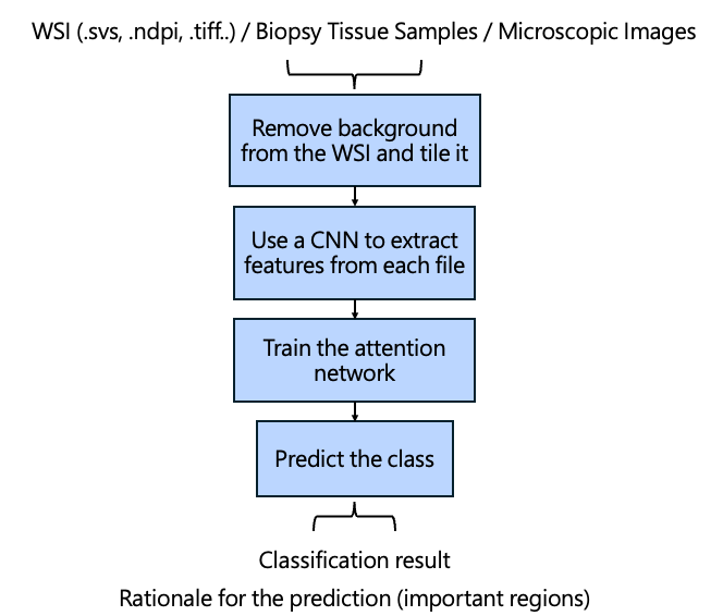Before training begins, the most crucial step is preprocessing the WSI, particularly because WSIs are extremely large and complex.

1. Patch Extraction & Feature Learning
CLAM first removes background and retains tissue regions. The WSI is then divided into 256 × 256 pixel patches, which are processed by a Convolutional Neural Network (CNN).

CNNs extract important features from tissue patches based on shape, color, and texture differences. These extracted features are encoded as lower-dimensional vectors, reducing the enormous amount of information in WSIs into compact representations.

2. Feature Projection & Attention Network
After preprocessing, the model begins training. Each WSI is now represented by k patches with extracted feature vectors zₖ. In the first layer (W₁), each zₖ is projected to a 512-dimensional feature vector hₖ using fully connected layers.

CLAM uses a multi-branch attention network, with each branch corresponding to one of the N classes. Each branch contains:

• An attention mechanism that computes attention scores aᵢ,ₖ for every patch k under class i

• A classifier Wcᵢ that predicts the class probability

A higher attention score aᵢ,ₖ indicates that patch k is more important for determining class i.

The model aggregates attention scores across all patches of a WSI to obtain the final class prediction.

3. Instance-level Refinement via Reinforcement

CLAM also incorporates a refinement mechanism: For each class i, the patches with the highest and lowest attention scores are used to train an auxiliary binary classifier. This helps the model better distinguish between patches belonging or not belonging to class i, strengthening decision boundaries.

Model Optimization

To evaluate performance, CLAM divides the dataset into a training set and a validation set. During validation, CLAM computes prediction errors using a loss function and adjusts the model accordingly.

CLAM uses multi-class SVM loss (Equation 1), where:

• \(s_y\) is the score for the true class
• \(\sum_j s_j\) is the sum of scores for other classes

When the margin between true and other classes exceeds a constant, the loss becomes zero, indicating good classification.

To improve stability, CLAM applies temperature scaling to create a smooth SVM loss, which provides smoother gradients for more robust neural network optimization.

During training:

• The number of epochs (typically 50–200) determines how many times the model repeats the training → validation → evaluation loop.

• The learning rate controls how much model weights update per step.

• CLAM uses the Adam optimizer, which adaptively adjusts learning rates based on past gradients—ideal for large pathology image datasets.

Summary of CLAM Training Pipeline

1. Patch the WSI
2. Extract features via CNN
3. Train attention networks
4. Validate model performance
5. Select the best-performing parameters

Throughout this process, users only need to provide data and corresponding labels—CLAM handles the rest and outputs high-accuracy predictions.

Reference

Lu, M.Y., Williamson, D.F.K., Chen, T.Y. et al. Data-efficient and weakly supervised computational pathology on whole-slide images. Nat Biomed Eng 5, 555–570 (2021). https://doi.org/10.1038/s41551-020-00682-w